Lecture 7 Paper
Absolutely — this chapter is a very important foundation for control engineering, and I’ll make it clear, structured, and beginner-friendly for you.
This file covers PID control: what it is, how it behaves, and why each term matters. It is one of the most important topics in process control.
Chapter 7 — PID Control: Characteristics, Forms, and Modes
Big Picture: What is PID control?
PID stands for:
- P = Proportional
- I = Integral
- D = Derivative
A PID controller continuously adjusts a system output so that it follows a desired target value (called the setpoint).
For example:
- desired room temperature = 22°C
- measured temperature = 20°C
- error = 2°C
The controller uses this error to decide how strongly to react.
The basic idea is:
\text{error} = \text{setpoint} - \text{measured output}
The controller uses this error in three different ways.
Why do we need PID?
The main purpose is to keep a process stable and accurate.
Examples:
- temperature control
- speed control
- liquid level control
- pressure control
- motor position control
The chapter states the key goals clearly:
- maintain stability
- minimize deviation from setpoint
- reject disturbances
- remove steady-state error (offset)
This is the heart of automatic control.
7.1 Introduction
This section introduces feedback control loops.
A feedback loop means:
- measure output
- compare with desired value
- calculate error
- adjust input
- repeat continuously
This loop happens constantly.


Think of a shower:
- setpoint = desired water temperature
- sensor = your skin
- controller = your brain
- actuator = your hand turning the tap
This is actually a real feedback system.
Very nice practical example.
7.2 Closed-Loop Transfer Functions
This is one of the most important theory sections.
Here they derive the mathematical behavior of the closed-loop system.
What is closed-loop?
Closed-loop means the output is measured and fed back.
Unlike open-loop:
- open-loop = no correction
- closed-loop = self-correcting
The block diagram on page 5 is extremely important.
It shows:
- controller
- actuator
- process
- sensor
- disturbance


Main transfer function
The key result is the classic closed-loop equation:
G_(s)=\frac{\text{forward path}}{1+\text{loop gain}}
This appears in the chapter as:
G_(s)=\frac{\prod(\text{input-output})}{\prod(\text{loop})+1}
This is the most important control equation in the chapter.
Why is this important?
Because it tells us:
- stability
- speed
- oscillation
- damping
- overshoot
Everything about dynamic behavior comes from this.
Characteristic equation
This is extremely important.
The denominator:
\text{Loop}(s)+1=0
is called the characteristic equation
The roots of this equation are the poles.
The poles determine system behavior.
Pole interpretation
This part is essential:
Negative real poles
Stable response
Output settles nicely.
Positive real poles
Unstable response
Output grows without bound.
Complex poles
Oscillatory response
You get overshoot and ringing.
This is the core theory behind stability.
Example 7.1 — P-only controller on second-order process
This example shows how proportional control affects system dynamics.
The result shows:
- underdamped behavior
- some overshoot
- faster response
This is exactly what proportional control usually does.
It speeds up response but may introduce oscillation.
Example 7.2 — Positive feedback
This is very important conceptually.
Normally PID uses negative feedback.
Negative feedback reduces error.
Positive feedback does the opposite.
It amplifies error.
That is why the system becomes unstable.
The chapter shows poles with positive real part.
That means instability.
Very important intuition:
- negative feedback = stabilizing
- positive feedback = destabilizing
Example 7.3 — Stabilizing an unstable process
This is a very nice example.
Sometimes the plant itself is unstable.
But with sufficient controller gain:
K_c > 1
the closed-loop system can become stable.
This is one of the great powers of feedback control.
It can stabilize an unstable process.
Example 7.4 — Routh stability criterion
This section is very important for exams.
They use Routh criterion to determine when the system is stable.
The idea:
Instead of solving all roots directly, we analyze the polynomial coefficients.
This tells us the stability limit.
Very commonly used in control theory.
7.3 Analysis of P, I and D Action
This is the heart of the chapter.
Now they explain each PID term individually.
1) Proportional control (P)
This is the simplest controller.
u(t)=K_c e(t)
u(t)=K_c e(t)
This means:
control action is directly proportional to current error
If error is large → large response
If error is small → small response
Intuition
Imagine driving a car.
If you are far from the lane center, you turn the wheel more.
That is proportional control.
Advantages
- fast
- simple
- easy to implement
Main weakness: offset
This is extremely important.
P-control usually leaves steady-state error
Also called:
- offset
- residual error
The system may settle close to target but not exactly at target.
This is shown clearly in the figure on page 11.
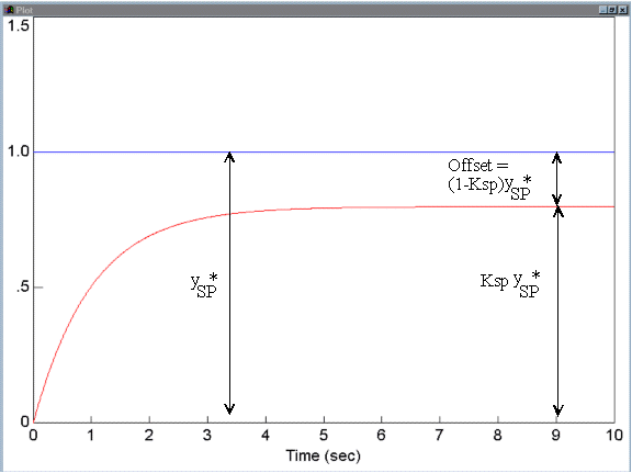

This is the major weakness of pure P control.
2) Integral control (I)
Integral action accumulates past error.
u(t)=K_c\frac{1}{\tau_i}\int e(t),dt
u(t)=K_c\frac{1}{\tau_i}\int e(t),dt
This means:
if error remains for a long time, the controller keeps increasing correction.
Why is this useful?
Because it removes offset.
This is the biggest advantage.
The chapter explicitly says:
eliminates offset
This is the key exam point.
Intuition
If temperature stays slightly below target for several minutes, the controller “remembers” this and keeps pushing harder.
Weakness
Too much integral action causes:
- overshoot
- oscillation
- slower settling
This is called integral windup tendency in practice.
3) Derivative control (D)
Derivative action responds to rate of change
u(t)=K_c\tau_D\frac{de(t)}{dt}
u(t)=K_c\tau_D\frac{de(t)}{dt}
This means it predicts where the error is going.
Intuition
Think of braking before a sharp turn.
You react not only to current position, but to how fast you are moving.
That is derivative control.
Main benefit
Derivative reduces oscillations.
It improves damping.
It acts like a prediction term.
Very important point from page 14:
reduces oscillatory nature
Weakness
Derivative is very sensitive to noise.
Because noise changes rapidly.
So D-control can amplify measurement noise.
This is why in real systems D is often filtered.
Summary of P, I and D
This table is the most important conceptual summary:
| Mode | Uses | Strength | Weakness |
|---|---|---|---|
| P | present error | fast | offset |
| I | past error | removes offset | oscillation/slower |
| D | future trend | damping/prediction | noise sensitive |
This is the essence of PID.
7.4 Position form of PID
This section gives the full controller equation
u(t)=\bar{u}+K_c\left(e(t)+\frac{1}{\tau_i}\int e(t)dt+\tau_D\frac{de(t)}{dt}\right)
u(t)=\bar{u}+K_c\left(e(t)+\frac{1}{\tau_i}\int e(t)dt+\tau_D\frac{de(t)}{dt}\right)
This is the standard PID formula.
Meaning of each term
- proportional = immediate correction
- integral = memory
- derivative = prediction
Together they create:
- speed
- accuracy
- damping
This is why PID is so widely used.
Derivative kick
Very important practical concept.
When setpoint changes suddenly, derivative term may spike strongly.
This is called derivative kick
The chapter explains this nicely.
Very common exam question.
7.5 Velocity form of PID
This form calculates change in output
Instead of controller output itself:
\Delta u(t)
This is useful in digital controllers and PLC systems.
Very common in industrial implementation.
7.6 Interactive form
This is an older analog controller representation.
Important mainly for historical and conversion purposes.
The chapter explains how parameters convert between:
- conventional PID
- interactive PID
Important if you work with older industrial systems.
Final intuition: why PID is powerful
PID works because it combines three perspectives:
- what is wrong now? → P
- what has been wrong for a while? → I
- where is it heading? → D
That is why it is so powerful.
Super short memory trick
- P = Present
- I = Past
- D = Future trend
This is honestly the easiest way to remember it.