Instrumentation

Lecture 6 Paper

Quiz ChatGPT conversation

Chapter 6: Dynamic Behavior of Ideal Systems

This chapter covers the most important “ideal” system models used in engineering and control:

ideal inputs
first-order systems
second-order systems
integrating systems
high-order systems
deadtime
FOPDT models

These are the core models used to approximate real industrial systems.

Examples:

tank level
reactor temperature
flow systems
chemical concentrations
mechanical systems

1) Idealized Process Inputs

Before understanding the system response, we first need to understand the types of input signals.

This is extremely important because the same system behaves differently depending on the input.

A) Impulse input

This is a very short but very strong input.

Imagine injecting dye instantly into a tank.

The input is almost like a spike:

huge magnitude
almost zero duration
finite total area

Visually:

one sharp vertical spike

The area under it equals 1 for a unit impulse.

Intuition

This is used to study how the system reacts to a sudden shock.

Examples:

sudden salt injection
pulse of energy
electrical spike

This is often used for system identification.

B) Step input

This is the MOST important input in control engineering.

A step means:

the input suddenly changes and stays there.

Example:

flow changes from 5 L/min → 8 L/min instantly

Like flipping a switch.

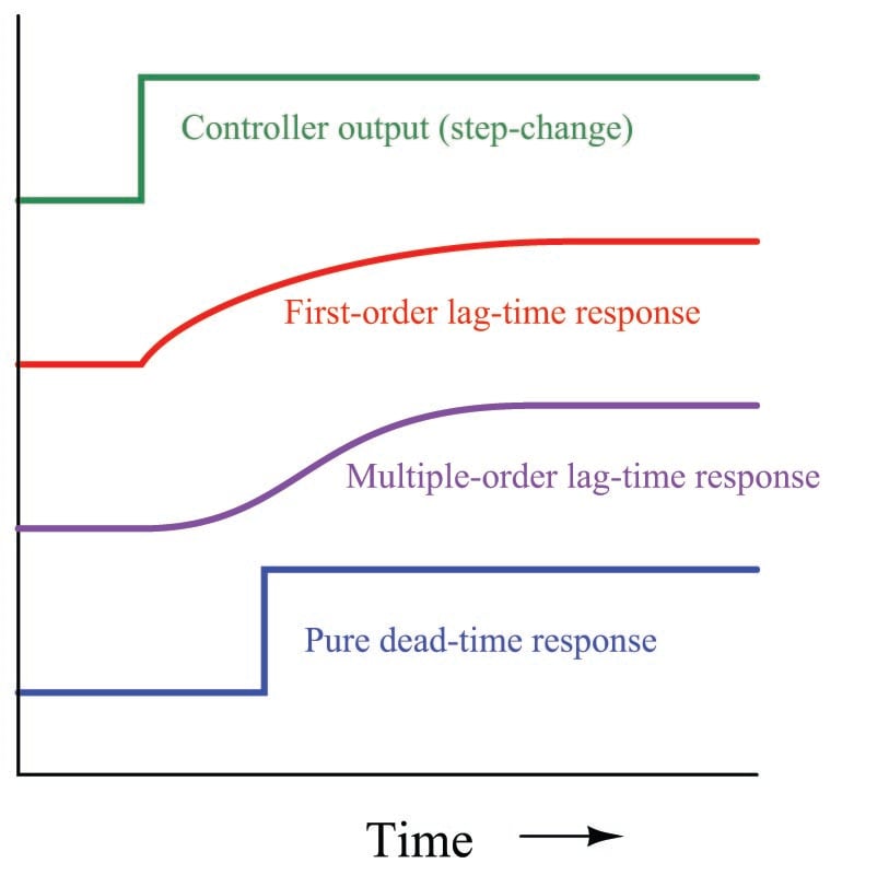
This is what most examples in the chapter use.

C) Pulse input

A pulse is like a temporary step.

Input rises suddenly, then returns back after some time.

Example:

inject salt for 5 seconds
stop injection

Very useful for tracer studies.

D) Ramp input

A ramp means the input increases continuously with time.

Example:

temperature increases steadily:

20°C → 25°C → 30°C → 35°C

This is common in industrial heating systems.

E) Sinusoidal input

This is periodic oscillation.

Like:

u(t)=A\sin(\omega t)

Examples:

day/night temperature cycles
AC electrical signals
vibration systems

This is very important in frequency response analysis.

2) First-Order Processes

This is probably the MOST important model in this chapter.

A first-order system has this differential equation:

\tau_p \frac{dy}{dt}+y=K_pu

Where:

(y(t)) = output
(u(t)) = input
(K_p) = process gain
(\tau_p) = time constant

What does this mean physically?

A first-order system responds smoothly and exponentially.

It does NOT jump instantly.

Instead it approaches the final value gradually.

Example:

tank heating
mixing concentration
simple RC circuits

Process gain (K_p)

This tells you how much output changes relative to input.

K_p=\frac{\Delta y}{\Delta u}

If gain is large → small input gives big output change

Time constant (\tau_p)

This is EXTREMELY important.

It tells how fast the system responds.

After 1 time constant:

63.2%

of the total change is completed.

63.2%

This is one of the most famous numbers in control systems.

Key memory points

After:

(1\tau) → 63.2%
(3\tau) → 95%
(4\tau) → 98%

This is VERY exam-relevant.

Step response of first-order system

For a step input:

y(t)=AK_p(1-e^{-t/\tau_p})

y(t)=AK_p\left(1-e^{-t/\tau_p}\right)

This gives the classic exponential rise curve.

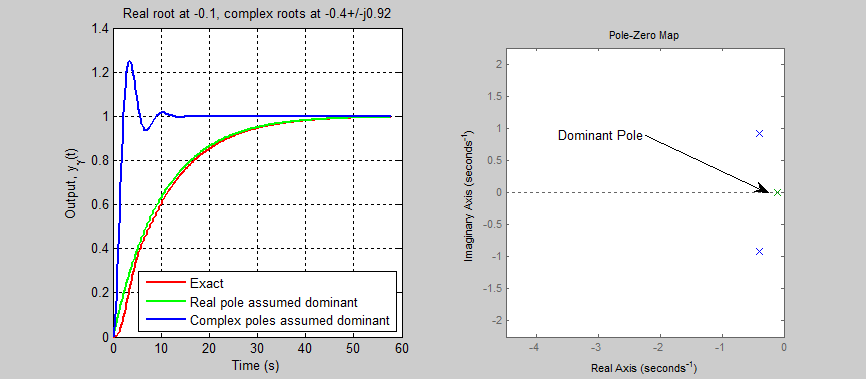
This curve is one of the most important in control theory.

3) Impulse response of first-order system

For an impulse:

y(t)=\frac{AK_p}{\tau_p}e^{-t/\tau_p}

Instead of rising, it starts high and decays exponentially.

This is commonly used in tracer experiments.

The reactor salt example in the chapter is a great real-life application.

4) Ramp response of first-order system

This is VERY important conceptually.

For ramp input, output also becomes ramp-like, but delayed.

The output follows with a lag.

At long times:

y(t)\approx aK_p(t-\tau_p)

Meaning:

the system behaves as if it is “late” by one time constant.

This is a powerful intuition.

5) Second-Order Processes

Now it gets more interesting.

Second-order systems can oscillate.

Equation:

\tau_n^2\frac{d^2y}{dt^2}+2\zeta\tau_n\frac{dy}{dt}+y=K_pu

Main parameters:

(K_p) = gain
(\tau_n) = natural period/time scale
(\zeta) = damping factor

MOST important: damping factor (\zeta)

This controls the shape of response.

Overdamped ((\zeta >1))

Slow response

No oscillation

Smooth approach

Critically damped ((\zeta=1))

Fastest possible response without oscillation

This is usually desirable.

Underdamped ((\zeta<1))

Oscillatory response

Overshoot + ringing

This is one of the most important concepts in dynamic systems.

6) Important second-order characteristics

These are very exam-relevant.

Rise time

Time required to first reach final value

Overshoot

How much the response exceeds the final value

Example: final = 10 peak = 12

overshoot = 20%

Decay ratio

Ratio of successive oscillation peaks

Shows how quickly oscillations disappear

Settling time

Time until response stays within ±5%

This is used a LOT in controller tuning.

7) Integrating processes

This is extremely important for tank level systems.

Equation:

\rho A_c\frac{dL}{dt}=F_-F_

Key idea:

the output keeps accumulating.

Example:

tank filling
charge storage
position from velocity

Why “integrating”?

Because output is the integral of input.

If inflow > outflow continuously

the level keeps rising forever

This is different from first-order systems which stabilize.

This is a HUGE conceptual difference.

8) High-order processes

These are systems with multiple time constants.

Example: distillation columns

Many trays → many first-order subsystems

Transfer function:

G(s)=\frac{K_p}{(\tau_ps+1)^n}

As (n) increases:

slower response
more sluggish
looks delayed

9) Deadtime

This is VERY important.

Deadtime means:

input changes now, but output changes later.

Example: temperature sensor far away from reactor

Transport delay

G(s)=e^{-\theta s}

genui{"math_block_widget_always_prefetch_v2":{"content":"G(s)=e^{-\theta s}"}}

This is common in industry.

Long pipes sampling delays measurement delays

10) FOPDT model

VERY VERY important.

First Order Plus Dead Time

G(s)=\frac{K_pe^{-\theta_ps}}{\tau_ps+1}

This is one of the most used industrial approximations.

Why?

Because real processes often behave like:

some delay
then smooth exponential response

This model captures both.

BIG picture summary

Think of the models like personalities:

first-order → smooth exponential
second-order → may oscillate
integrating → keeps accumulating
high-order → sluggish
deadtime → delayed response
FOPDT → delayed + smooth

This chapter is basically teaching you the “language” of control engineering.

Once you master these response shapes, later controller tuning becomes much easier.

Quiz

Score: 0/30 (0%)

Q0. In process dynamics, what is the main purpose of using idealized input signals such as step, impulse, ramp, and sinusoidal inputs?

To make real processes behave linearly at all times

To test and describe how a system responds to different types of changes over time

To eliminate deadtime from industrial systems

To replace the need for differential equations

Q1. Which description best matches a step input?

A sudden change in input that remains at the new value

A very short input with very large magnitude and finite area

An input that increases linearly with time

An input that repeatedly oscillates above and below zero

Q2. Which input type is best described as a brief, sharp disturbance with finite total effect?

Ramp input

Step input

Impulse input

Sinusoidal input

Q3. What is the defining behavior of a first-order process after a step input?

It immediately reaches the final value

It approaches the final value smoothly and exponentially

It always oscillates before settling

It keeps increasing forever

Q4. What does the process gain describe in a dynamic system?

How fast the system responds

How much the output changes relative to the input change

How much deadtime the system has

How many energy storage elements the system contains

Q5. What does the time constant of a first-order process mainly tell us?

The final value reached by the system

The amount of overshoot

How quickly the system responds

The number of oscillations before settling

Q6. For a first-order process responding to a step input, approximately how much of the total change has occurred after one time constant?

25.0%

50.0%

63.2%

95.0%

Q7. Which statement best distinguishes a first-order system from a second-order system?

A first-order system always has deadtime, while a second-order system does not

A first-order system has one dominant lag, while a second-order system has two interacting dynamic effects

A first-order system cannot reach steady state, while a second-order system always can

A first-order system only responds to impulse inputs, while a second-order system only responds to step inputs

Q8. Which second-order response type is usually considered the fastest response without oscillation?

Underdamped

Overdamped

Critically damped

Unstable

Q9. What is the main characteristic of an underdamped second-order system?

It responds instantly with no delay

It approaches the final value slowly without crossing it

It overshoots and oscillates before settling

It never responds to input changes

Q10. What does overshoot measure in a second-order step response?

How far the response goes beyond the final steady-state value

How long the input takes to change

How much deadtime occurs before the response begins

How many first-order systems are connected in series

Q11. What does settling time describe?

The time required for the input to reach its maximum

The time required for the system response to remain close to its final value

The time between two consecutive input pulses

The time required for an impulse input to disappear

Q12. Which process type is characterized by continuous accumulation when there is a persistent imbalance between input and output?

First-order process

Second-order process

Integrating process

Pure deadtime process

Q13. Which example is most representative of an integrating process?

A thermometer slowly reaching the surrounding temperature

A tank level rising because inflow is greater than outflow

A mass-spring system oscillating after a disturbance

A sensor responding after a transport delay

Q14. Why are high-order processes often approximated by simpler models?

Because high-order processes are always unstable

Because simple models can capture the dominant response behavior without needing every internal detail

Because high-order processes have no steady-state gain

Because deadtime cannot exist in high-order systems

Q15. What is deadtime in a dynamic process?

The time required for the output to reach 63.2% of its final value

A delay between an input change and the first visible output response

The time required for oscillations to disappear

The time required for the input to return to zero

Q16. What does an FOPDT model combine?

First-order behavior and deadtime

Second-order oscillation and impulse behavior

Ramp input and sinusoidal input

Integrator behavior and unstable feedback only

Q17. Why is the FOPDT model widely used in process control?

Because all industrial systems are exactly first order

Because it often gives a practical approximation of real processes using only gain, time constant, and deadtime

Because it removes the need for controller tuning

Because it only works for systems with no delay

Q18. Which statement best describes a ramp response of a first-order system?

The output follows the ramp perfectly with no lag

The output remains constant forever

The output follows the ramp but with a delay or lag

The output always oscillates around the ramp

Q19. Which feature is most associated with a sinusoidal input?

A sudden permanent change

A repeating periodic change

A one-time spike

A continuous linear increase

Q20. True or false: A first-order process always reaches its new steady state instantly after a step input.

True

False

Q21. True or false: The time constant of a first-order process is related to how fast the process responds.

True

False

Q22. True or false: After one time constant, a first-order process has completed approximately 63.2% of its total response to a step input.

True

False

Q23. True or false: Second-order systems can show overshoot and oscillation, depending on the damping.

True

False

Q24. True or false: An overdamped second-order system oscillates strongly before reaching steady state.

True

False

Q25. True or false: A critically damped system is the fastest ideal second-order response that avoids oscillation.

True

False

Q26. True or false: Integrating processes naturally settle to a new steady value after a constant imbalance in input and output.

True

False

Q27. True or false: Deadtime means that the output response begins before the input changes.

True

False

Q28. True or false: High-order processes often appear more sluggish than simple first-order processes.

True

False

Q29. True or false: An FOPDT model is useful because it combines a simple first-order response with a time delay.

True

False