Instrumentation

Lecture 5 Paper

Quiz ChatGPT conversation

Chapter 5 — Transfer Functions and State Space Models

This chapter is essentially about one big question:

How do we mathematically describe how a system responds over time when we change its input?

Examples:

changing valve opening → tank level changes
changing heater power → temperature changes
changing motor voltage → speed changes

This is the language of control engineering.

1) Big Idea: What is a Transfer Function?

The most important equation in this chapter is:

G(s)=\frac{Y(s)}{U(s)}

where:

(Y(s)) = output in Laplace domain
(U(s)) = input in Laplace domain
(G(s)) = transfer function

This means:

transfer function = output response / input signal

A transfer function tells us:

speed of response
overshoot
delay
stability
oscillation tendency

Think of it as the “personality” of the system.

Easy intuition

If input is:

heater power

and output is:

room temperature

then the transfer function describes:

how fast room heats
whether it overshoots
whether it stabilizes

2) Why Use Laplace Transform?

This is one of the most important conceptual points.

Instead of solving differential equations directly in time domain:

\frac{dy}{dt}

we transform them into algebraic equations in (s)-domain.

That turns difficult calculus into simple algebra.

For example:

\frac{dy}{dt}+\frac{1}{\tau}y=\frac{1}{\tau}u

becomes

sY(s)+\frac{1}{\tau}Y(s)=\frac{1}{\tau}U(s)

Much easier.

3) Deviation Variables (VERY Important)

This chapter spends a lot of time on this because it is fundamental.

A deviation variable means:

how much the variable changes from steady state

Formula:

\hat y = y-\bar y

\hat u = u-\bar u

Where:

(y) = actual output
(\bar y) = steady-state value
(\hat y) = deviation from steady state

Why do we use this?

Because control systems care about changes, not absolute values.

Example:

If tank level is normally 5 m and becomes 6 m:

\hat h = 6-5=1

So the system changed by +1 m

This makes equations cleaner.

4) First-Order System (Most Important Model)

This is probably the most important section for exams.

The basic first-order equation:

\frac{dy}{dt}=\frac{1}{\tau}(u-y)

This appears everywhere:

temperature systems
mixing tanks
concentration changes
motor speed

Meaning of (\tau)

\tau = \text{time constant}

This controls how fast the system responds.

Small (\tau):

fast response

Large (\tau):

slow response

Transfer function of first-order system

After Laplace transform:

G(s)=\frac{1}{\tau s+1}

This is probably the single most important formula in this chapter.

G(s)=\frac{1}{\tau s+1}

5) Step Response (SUPER Important)

A step input means sudden change.

Example:

heater power suddenly changes from 0 → 100%

Mathematically:

U(s)=\frac{A}{s}

Then output becomes:

y(t)=A(1-e^{-t/\tau})

y(t)=A\left(1-e^{-t/\tau}\right)

What does this mean?

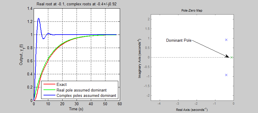
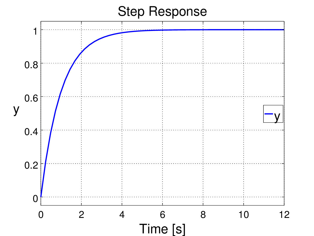
This gives the classic exponential rise curve.

Starts fast, then slowly levels off.

This is the classic response curve you see everywhere in control systems.

Important rule

At:

t=\tau

system reaches about:

63.2%

of final value

VERY commonly tested.

6) Impulse Response

Impulse means a very fast sudden pulse.

Input:

U(s)=1

Output:

y(t)=\frac{1}{\tau}e^{-t/\tau}

This is useful for analyzing system dynamics.

7) Ramp Response

Ramp means linearly increasing input.

Example:

temperature setpoint continuously rising

U(s)=\frac{B}{s^2}

Output:

y(t)=Bt-B\tau(1-e^{-t/\tau})

This shows lag behind changing inputs.

8) PID Controller Transfer Function

This is one of the most important applied parts.

PID equation:

c(t)=K_c\lefte(t)+\frac{1}{\tau_I}\int e(t)dt+\tau_D\frac{de}{dt}\right

Transfer function:

G_c(s)=K_c\left(1+\frac{1}{\tau_I s}+\tau_D s\right)

Meaning of each term

P = proportional

Responds to current error

I = integral

Removes steady-state offset

D = derivative

Predicts future trend / dampens oscillation

This is extremely important in process control.

9) Block Diagrams

This section is very practical.

A block diagram visually shows signal flow.

Example:

Input → controller → process → sensor → output

Series blocks

When blocks are connected in series:

G_(s)=G_1(s)G_2(s)G_3(s)

VERY important rule.

You simply multiply them.

Why?

Because intermediate signals cancel.

This makes large systems much easier to analyze.

10) Linearization of Nonlinear Systems (VERY Important)

This is one of the hardest but most useful sections.

Real systems are often nonlinear.

Example:

\frac{dy}{dt}=f(y,u)

Nonlinear equations are difficult.

So we approximate them near an operating point using Taylor expansion.

Main idea

Approximate nonlinear curve by tangent line locally.

This is exactly what linearization means.

f(y,u)\approx f(\bar y,\bar u)+ (y-\bar y)\frac{\partial f}{\partial y}+ (u-\bar u)\frac{\partial f}{\partial u}

This is extremely important.

11) Tank Level Example

Very exam-relevant example.

Nonlinear equation:

F_=C_v\sqrt{h}

This is nonlinear because of square root.

To linearize:

\sqrt h \approx \sqrt{\bar h}+\frac{1}{2\sqrt{\bar h}}(h-\bar h)

\sqrt{h}\approx \sqrt{\bar h}+\frac{1}{2\sqrt{\bar h}}(h-\bar h)

This is classic first-order Taylor expansion.

Why is this useful?

Because after linearization we can use:

Laplace transform
transfer functions
controller design

This is a huge concept in control engineering.

12) Important Practical Insight

The chapter makes an excellent point:

Linear models work best close to operating point

Far away → errors become large

This is shown in the tank example where nonlinear and linear models start to differ.

This is very important conceptually.

Final Big-Picture Summary

This whole chapter teaches:

How systems react to inputs over time

Main tools:

deviation variables
Laplace transforms
transfer functions
block diagrams
linearization

Core formulas to remember:

G(s)=\frac{Y(s)}{U(s)}

G(s)=\frac{1}{\tau s+1}

G_c(s)=K_c\left(1+\frac{1}{\tau_I s}+\tau_D s\right)

What you should absolutely memorize

transfer function definition
first-order transfer function
step response
time constant meaning
series blocks multiply
PID transfer function
Taylor linearization idea

These are almost always tested.

Quiz

Score: 0/31 (0%)

Q0. What is the main purpose of using a transfer function in process control?

To describe the relationship between an input and an output in the Laplace domain

To measure the physical size of a process unit

To eliminate the need for experimental data

To describe only nonlinear systems in their original form

Q1. Why are deviation variables often used when deriving transfer functions?

They make all nonlinear systems exactly linear

They express variables as changes from their steady-state values

They remove the need for Laplace transforms

They convert time-domain equations into frequency-domain graphs automatically

Q2. Which statement best describes a first-order system?

A system that responds instantly to any input change

A system whose output oscillates forever after a disturbance

A system that gradually approaches a new steady-state value after an input change

A system whose output always increases without limit

Q3. What does the time constant of a first-order system mainly indicate?

The final steady-state value of the system

How fast or slow the system responds

The amount of noise in the measurement

The number of inputs in the model

Q4. In a first-order step response, what does the output typically do after a sudden input change?

It jumps immediately to the final value

It approaches the final value gradually

It decreases forever

It oscillates with constant amplitude forever

Q5. What is an integrating system?

A system that always returns to its original value after a disturbance

A system that accumulates input over time

A system that only works with digital signals

A system that has no dynamic behavior

Q6. Which example best represents an integrating process?

A thermometer approaching room temperature

A capacitor discharging through a resistor

The level in a tank increasing when inflow exceeds outflow

A spring returning to its equilibrium position

Q7. How does an integrating system differ from a typical first-order self-regulating system?

An integrating system naturally settles faster

An integrating system accumulates input and may not settle without balance or control

A first-order system cannot be modeled mathematically

A first-order system always has no steady state

Q8. What is the purpose of linearization in process modeling?

To replace a nonlinear system with an approximate linear model near an operating point

To remove all process dynamics from the model

To make the model valid for every possible operating condition

To convert a transfer function back into a nonlinear differential equation

Q9. Why is linearization usually only locally valid?

Because it is based on an approximation around a chosen operating point

Because it only works for systems with no inputs

Because Laplace transforms cannot be used with linear models

Because all real systems are exactly linear only at high temperatures

Q10. In a block diagram, what happens to transfer functions connected in series?

They are subtracted

They are divided by the input

They are multiplied

They are ignored

Q11. What does a block diagram help engineers understand?

Only the physical layout of pipes and valves

The flow of signals and dynamic relationships between parts of a control system

The chemical composition of the process fluid

The cost of each process unit

Q12. What is the role of the proportional part of a PID controller?

It reacts to the current error

It only reacts to accumulated past error

It only reacts to the future predicted error

It removes all system dynamics

Q13. What is the main role of the integral part of a PID controller?

To increase measurement noise

To remove steady-state offset by accumulating error over time

To predict the slope of the error only

To make the process nonlinear

Q14. What is the main role of the derivative part of a PID controller?

To respond to the rate of change of error

To accumulate all previous errors

To make the controller independent of the process

To force the output to increase forever

Q15. A transfer function describes the relationship between input and output in the Laplace domain.

True

False

Q16. Deviation variables describe absolute process values rather than changes from steady state.

True

False

Q17. A first-order system usually approaches a new steady state gradually after a step change.

True

False

Q18. A smaller time constant means a slower first-order response.

True

False

Q19. An integrating system accumulates the effect of input over time.

True

False

Q20. An integrating process always naturally returns to a fixed steady state after a constant input disturbance.

True

False

Q21. Linearization means approximating nonlinear behavior with a linear model near an operating point.

True

False

Q22. A linearized model is usually accurate for all possible operating conditions.

True

False

Q23. Block diagrams can be used to represent controllers, processes, sensors, and feedback paths.

True

False

Q24. Transfer functions in series are combined by multiplying them.

True

False

Q25. The proportional term in a PID controller responds to accumulated past error.

True

False

Q26. The integral term of a controller can help remove steady-state offset.

True

False

Q27. The derivative term responds to how quickly the error is changing.

True

False

Q28. Laplace transforms are useful because they can turn differential equations into algebraic equations.

True

False

Q29. A nonlinear tank outflow relationship such as square-root dependence can be approximated linearly near a chosen steady-state level.

True

False

Q30. A first-order model is useful because many real process variables, such as temperature, concentration, or tank level with resistance, respond gradually rather than instantly.

True

False