Instrumentation

Lecture 7 PPT

Quiz ChatGPT conversation

Lecture Summary: Stability and P-Control

Topic: Controller Design, Stationary Error, Proportional Control

This lecture is one of the core foundations of control engineering. The main question throughout is:

How do we make a system behave the way we want?

For example:

follow a desired temperature 🌡️
keep motor speed constant ⚙️
reduce disturbances 🔇
make the response faster ⚡

Page 1 — Introduction

Controller design

stationary errors
proportional control
P control

This is the roadmap of the lecture.

Main focus:

Understand stability
Understand steady-state (stationary) error
Learn the simplest controller: P-controller

Page 2 — Control Purposes 🎯

This page explains why we use control systems.

There are 4 main goals:

1) Follow a reference

The output should follow what we ask it to do.

Example: If we want temperature = 50°C, the system should reach 50°C.

This is written as:

\frac{Y(s)}{R(s)}

Where:

(R(s)) = reference/input
(Y(s)) = output

This ratio tells us how well output follows input.

2) Dampen noise and disturbances

Real systems are never perfect.

There can be:

external disturbances
sensor noise
random fluctuations

Example: wind affecting a drone ✈️

The system must reduce their effect.

This is:

\frac{Y(s)}{W(s)}

Where (W(s)) = disturbance/noise

3) Stabilize the system

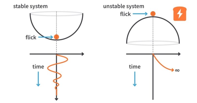
A system must not oscillate forever or explode.

Bad example:

output keeps increasing infinitely
oscillation gets larger and larger

Good system:

settles nicely

4) Faster response ⚡

A system that takes 20 minutes to respond is usually bad.

We want:

fast rise
quick settling

Page 3 — Closed Loop Transfer Function 🔁

This is one of the most important equations.

\frac{Y(s)}{R(s)}= \frac{D(s)G(s)} {1+D(s)G(s)H(s)}

Let’s break it down.

Meaning of blocks

(D(s))

Controller

This is what we design

Example: P-controller

D(s)=K

(G(s))

Plant/system

This is the physical system:

motor
heater
robot arm

(H(s))

Sensor/feedback

Measures output and sends it back.

This whole equation describes the closed-loop behavior.

Page 4 — Following a Reference

This page introduces:

Closed-loop transfer

T(s)=\frac{Y(s)}{R(s)}

Open-loop transfer

L(s)=D(s)G(s)H(s)

Most important:

Characteristic equation

1+D(s)G(s)H(s)=0

This equation determines the poles.

Poles determine:

stability
speed
oscillation

Very important concept.

Page 5 — Characteristic Equation and Stability ⚠️

This page explains poles.

The roots of:

1+D(s)G(s)H(s)=0

are the system poles.

Important rule

For stability, poles must have negative real parts

That means:

s=-1,,-2

is stable ✅

But:

s=+1

is unstable ❌

Intuition

Negative poles = output decays and settles

Positive poles = output grows

This is extremely important in control.

Page 6 — First-Order System 📈

Very important system:

\frac{Y(s)}{R(s)}= \frac{K}{\tau s+1}

Meaning

(K)

Gain Final amplification

(\tau)

Time constant

This controls speed

Smaller (\tau) = faster system ⚡

63% rule ⭐

After one time constant (\tau), output reaches:

63%

of final value

This is a classic rule.

Very important for exams.

Pole

-\frac{1}{\tau}

Again:

smaller (\tau) → pole further left → faster

Page 7 — Second-Order System 🌊

Now system becomes:

\frac{\omega_n^2} {s^2+2\zeta\omega_n s+\omega_n^2}

This is much more realistic.

Many real systems behave like this.

Important parameters

(\omega_n)

Natural frequency

Controls speed

(\zeta)

Damping ratio

Controls overshoot and oscillation

Response properties

Rise time

How fast it first reaches target

Peak time

Time until maximum overshoot

Settling time

Time until it stays near final value

Overshoot

How much it exceeds target

Example: Target = 1 Maximum = 1.2

Overshoot = 20%

Page 8 — Second Order Roots

Uses quadratic formula:

x= \frac{-b\pm \sqrt{b^2-4ac}}{2a}

Cases

(b^2-4ac>0)

Two real poles

Usually no oscillation

(=0)

Repeated poles

Critical damping

(<0)

Complex poles

Oscillatory behavior 🌊

Page 9 — Complex Poles

Example:

x^2+2x+5=0

Solution:

x=-1\pm 2j

Meaning

Real part = (-1)

Imaginary part = (\pm2)

This gives oscillation that decays over time.

Because real part is negative.

Page 10 — Pole Placement 🧭

This image is extremely important.

It shows pole locations in the complex plane.

Left side = stable ✅

Negative real part

Right side = unstable ❌

Positive real part

Complex poles

Oscillation

Further left = faster decay

Higher imaginary = more oscillation

Page 11 — Overshoot and Pole Angle 📐

Very important idea.

Small angle → high overshoot

Large angle → low overshoot

When angle approaches 90°:

poles become real
no overshoot

This slide links pole location to response shape

Very important concept.

Pages 12–20 — Steady-State Error / Stationary Error 🎯

This whole section is about:

Does output exactly reach reference?

This is called:

steady-state error

Definition

e(\infty)=r(\infty)-y(\infty)

Difference between desired and actual output after long time.

Example: Reference = 1 Output = 0.9

e_=0.1

System Type ⭐

Very important exam concept.

System type = number of poles at zero

Example:

Type 0: \frac{5}{(s+1)(s+10)}

No pole at zero

Type 1: \frac{5}{s(s+10)}

One pole at zero

Type 2: \frac{5}{s^2(s+10)}

Two poles at zero

Important Rules Table ⭐⭐⭐

For step input

Type 0 → finite error
Type 1 → zero error
Type 2 → zero error

For ramp input

Type 0 → infinite error
Type 1 → finite error
Type 2 → zero error

For parabolic

Type 0 → infinite
Type 1 → infinite
Type 2 → finite

This is one of the most important pages.

Page 21 — Visual Comparison 📊

This image slide is excellent.

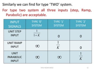
It visually shows:

More integrators → less stationary error

This is a key intuition.

Page 23–24 — PID Introduction ⚙️

Now lecture moves to controllers.

Most common controller:

PID

P = proportional
I = integral
D = derivative

Today’s lecture focuses only on P

Page 25 — Proportional Control ⭐

Very important slide.

D(s)=K

This means controller is just a constant gain.

Control law

U(s)=K\cdot E(s)

Where:

(E(s))=error
(U(s))=control signal

Meaning

Bigger error → bigger correction

Simple and intuitive.

Example: If temperature is too low, heater power increases.

Page 26 — Closed Loop with P Control

This is the core derivation.

For first-order system:

G(s)=\frac{K_s}{\tau s+1}

with controller:

D(s)=K_c

Closed loop becomes:

\frac{K_cK_s} {\tau s+1+K_cK_s}

Key conclusion ⭐

Larger (K_c):

faster response
smaller time constant
smaller error

This is extremely important.

Pages 27–31 — Example I 🚀

Practical example:

G(s)=\frac{7}{s+7}

This is first-order.

Goal

Make system faster

By increasing:

K_c

Result

Time constant becomes smaller

Example: \tau=\frac{1}{7}

With (K_c=1)

\tau_=\frac{1}{14}

Twice as fast ⚡

But...

There is still stationary error.

Important limitation of P-control.

Large (K_c)

When (K_c=10) or 100:

response becomes very fast
error becomes very small

BUT control signal becomes huge ⚠️

This may damage actuator in real life.

Very important engineering tradeoff.

Pages 32–35 — Example II 🌊

Now second-order system:

G(s)=\frac{1}{s(s+1)}

Goal:

limited output
no overshoot

Characteristic equation:

s^2+s+K=0

Key result

For real poles:

K\le0.25

This is very important.

If K becomes too large:

poles become complex
overshoot appears

Pages 36–37 — Noise Reduction 🔇

Excellent practical section.

Disturbance transfer:

[ \frac{Y(s)}{W(s)}

\frac{1}{1+G(s)H(s)D(s)} ]

Important intuition

Bigger controller gain reduces disturbance effect

Because denominator gets larger.

This is one major advantage of feedback control.

Page 38 — Final Summary ⭐⭐⭐

Perfect summary slide.

P-control advantages

easy
often stabilizes system
improves speed
reduces stationary error

Limitation ⚠️

If no integrator exists, stationary error remains

This is one of the most important conclusions.

P-control improves error

but often cannot eliminate it completely.

That is why later lectures use:

Big Picture Summary 🧠

The lecture teaches:

Stability depends on poles
Pole placement determines dynamics
System type determines steady-state error
P-control makes systems faster
P-control reduces but may not remove stationary error

This is really one of the most important foundational control lectures.

The next natural step is usually PI control, where integral action removes stationary error completely.

Quiz

Score: 0/31 (0%)

Q0. What is the main purpose of a closed-loop control system?

To remove the controller from the system

To make the output follow a reference, reduce disturbances, stabilize the system, and improve response speed

To make the system independent of feedback

To ensure the system always has zero overshoot

Q1. In the closed-loop transfer function Y(s)/R(s) = D(s)G(s)/(1 + D(s)G(s)H(s)), what does D(s) represent?

The physical process or plant

The sensor

The controller

The disturbance input

Q2. What is the characteristic equation of a standard feedback control system?

D(s)G(s) = 0

1 + D(s)G(s)H(s) = 0

Y(s)/R(s) = 0

G(s)H(s) = R(s)

Q3. Why are the roots of the characteristic equation important?

They determine only the final value of the input

They determine the poles of the system and therefore stability and dynamic behavior

They determine the sensor type only

They determine whether the controller is physically large

Q4. For a stable continuous-time system, where should the poles be located?

On the positive real side of the complex plane

Only on the imaginary axis

In the left half-plane, meaning they have negative real parts

Anywhere as long as the imaginary part is zero

Q5. For a first-order system K/(τs + 1), what does τ represent?

The steady-state error

The natural frequency

The time constant

The damping ratio

Q6. Approximately how much of its final value has a first-order system reached after one time constant τ?

10%

37%

63%

100%

Q7. In a second-order system, what does the damping ratio ζ mainly influence?

The amount of overshoot and oscillation

The number of sensors

The reference signal amplitude only

The system type only

Q8. For the quadratic equation ax² + bx + c = 0, what happens when b² - 4ac < 0?

There are two real distinct roots

There are two equal real roots

There are complex conjugate roots

There are no poles

Q9. For the equation x² + 2x + 5 = 0, the roots are -1 ± 2j. What does the negative real part indicate?

The system response grows without limit

The oscillation is completely absent

The oscillatory response decays over time

The system has no dynamic behavior

Q10. What does a small pole angle α in the second-order pole placement diagram correspond to?

High overshoot

No overshoot

A pure integrator

A type 0 system

Q11. What is steady-state error?

The maximum overshoot of the output

The difference between reference and output as time approaches infinity

The initial value of the controller output

The imaginary part of the dominant pole

Q12. For unity feedback, what is the transfer function between E(s) and R(s)?

E(s)/R(s) = G(s)/(1 + G(s))

E(s)/R(s) = 1/(1 + G(s))

E(s)/R(s) = 1 + G(s)

E(s)/R(s) = G(s)

Q13. In control systems, what does system type refer to?

The number of sensors in the loop

The number of poles at the origin, meaning the number of integrations

The number of zeros in the numerator

The number of reference inputs

Q14. For a proportional controller, what is D(s)?

D(s) = Ks

D(s) = K/s

D(s) = K

D(s) = s/K

Q15. A proportional controller produces an output U(s) that is proportional to the error E(s).

True

False

Q16. Increasing the proportional gain Kc in a first-order closed-loop system can make the system respond faster.

True

False

Q17. A larger proportional gain always eliminates steady-state error in a type 0 system.

True

False

Q18. If a system has one pole at s = 0, it is called a type 1 system.

True

False

Q19. A type 0 system has zero steady-state error for a unit step input.

True

False

Q20. For a unity feedback type 0 system, the steady-state error for a unit step input is ess = 1/(1 + Kp).

True

False

Q21. Complex conjugate poles always have opposite real parts.

True

False

Q22. A second-order system with complex poles can show overshoot.

True

False

Q23. If the poles are real and negative, the system can be stable without oscillatory overshoot.

True

False

Q24. In Example I, the system G(s) = 7/(s + 7) is a first-order system.

True

False

Q25. For Example I, using proportional control with Kc = 1 makes the closed-loop time constant smaller than the open-loop time constant.

True

False

Q26. In Example II, G(s) = 1/[s(s + 1)] already contains an integrator.

True

False

Q27. For Example II with proportional control, the characteristic equation is s² + s + K = 0.

True

False

Q28. For Example II, real closed-loop poles occur when K is greater than 0.25.

True

False

Q29. The disturbance transfer function Y(s)/W(s) = 1/[1 + G(s)H(s)D(s)] shows that feedback can reduce the effect of disturbances.

True

False

Q30. P control is always sufficient to solve every control problem.

True

False