Dynamic Response of Second-Order Systems, Time Delay, Discretization & Simulation

This lecture is really about one big question:

“If I know the input to a system, what output will I get over time?”

This is the heart of process control, chemical engineering, biological systems, and automation.

Examples:

• heater power → temperature
• pump voltage → tank level
• flow → concentration
• pressure valve → pressure

The key idea is that systems do not react instantly.

They respond dynamically over time.

Page 1–2: Overview / Agenda

The lecture covers four major themes:

1) Dynamic response of systems

How systems respond when you suddenly change the input.

Especially:

• first-order systems
• second-order systems
• systems with delay

2) Discretization

How to convert continuous equations into step-by-step calculations.

This is super important for computers.

Because computers calculate:

one time step at a time

instead of continuous mathematics.

3) Inverse problem

Instead of asking:

what output do I get from an input?

we ask:

what input do I need to get a desired output?

Very important in control engineering.

4) Matlab simulation

How to simulate all this numerically.

Page 3: Modelling

This is one of the most important slides.

The system is represented as:

u(t) \rightarrow G(s) \rightarrow y(t)

Where:

• (u(t)) = input
• (y(t)) = output
• (G(s)) = system model / transfer function

Important concept

The output depends on:

• current input
• previous input
• system memory

This is the key difference from simple algebra.

Example:

A heater does not instantly reach temperature.

It remembers previous heating.

This memory is what differential equations describe.

Page 4: Ideal Systems

Very important theoretical idea.

Real systems are complicated.

Instead of modelling every tiny physical detail, we use ideal mathematical models.

Examples:

• first-order
• second-order
• integrating
• delayed
• FOPDT

These capture the essential behavior.

This is exactly what engineers do in practice.

Page 5: First-Order System

This is one of the most important models.

\tau_p \frac{dy(t)}{dt}+y(t)=K_pu(t)

This describes systems like:

• temperature change
• concentration mixing
• drug diffusion
• capacitor charging

What do the parameters mean?

(K_p): gain

K_p = \frac{\Delta y}{\Delta u}

This tells how much output changes for a given input change.

Example:

If heater power increases by 2 units and temperature rises by 10°C

K_p=5

(\tau): time constant

Extremely important.

This tells how fast the system responds.

After one time constant:

63%

of the final response is reached.

That 63% rule is essential.

Step response

For step input:

u(t)=1

the output is:

y(t)=AK_p(1-e^{-t/\tau})

This gives the classic exponential rise.

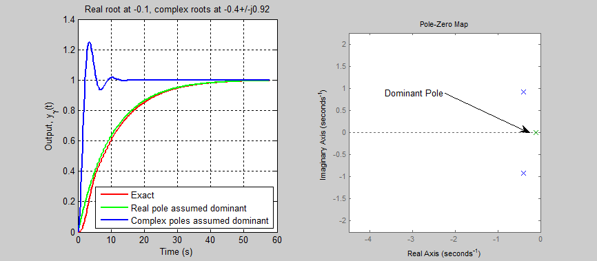
This curve is everywhere in engineering.

Page 6: Integrating System

This is another major system type.

Very important.

Transfer function contains:

\frac{1}{s}

This means:

the output accumulates input over time

Physical meaning

Perfect example:

tank level

If water enters continuously, level keeps increasing.

The system integrates flow.

\text{level}=\int \text{flow},dt

This is why tanks are classic integrators.

Key intuition

Constant input → linearly increasing output

Unlike first-order systems, it does not settle automatically.

That’s very important.

Page 7: Linearized System

This is extremely important theoretically.

Real systems are often nonlinear.

Example:

• pumps
• enzyme kinetics
• biological growth

But around a working point, we approximate them as linear.

This is called:

linearization

You asked about this earlier, so here’s the intuition again:

We zoom in near one operating point.

Locally, nonlinear curve ≈ straight line.

Like approximating a curved road as straight if you only look at 2 meters.

This makes control mathematically manageable.

Page 8: Nonlinearity Example (Pump)

Excellent practical example.

A pump needs minimum voltage before it even starts moving.

Because of friction.

So even when controller says:

u=0.5

nothing happens.

This is a dead zone / offset nonlinearity

Very realistic.

The controller adds offset voltage to overcome friction.

Very common in motors and pumps.

Page 9–10: Second-Order Systems

This is one of the most important topics.

Equation:

\tau_n^2\frac{d^2y}{dt^2}+2\zeta\tau_n\frac{dy}{dt}+y=K_pu(t)

Second derivative means:

system has inertia + momentum

Examples:

• mechanical systems
• fluid systems
• tanks + controller
• oscillations

Important parameters

(K_p)

steady-state gain

(\tau_n)

natural period / speed

Controls how fast oscillation happens.

(\zeta)

damping factor

This is SUPER important.

Controls overshoot and oscillation.

Page 11–12: Damping Behavior

This is probably the most important concept in second-order systems.

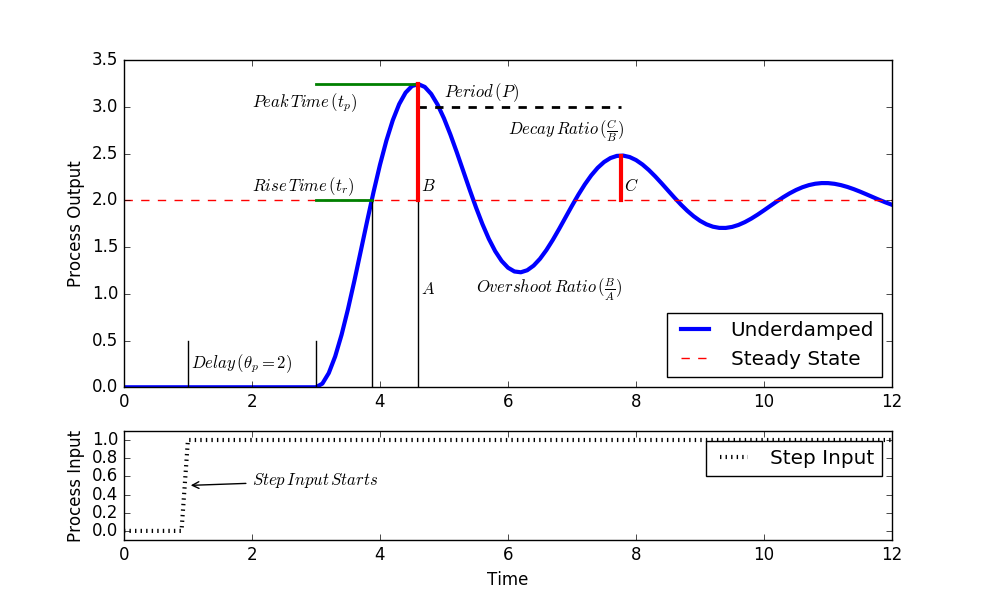
Underdamped

0<\zeta<1

System oscillates.

Overshoot happens.

Classic “ringing” response.

Critically damped

\zeta=1

Fastest response without overshoot.

Often ideal in control systems.

Overdamped

\zeta>1

Very smooth.

No oscillation.

But slower.

Important insight

Complex poles = oscillation

This is one of the most exam-important statements.

Page 13: Rise Time

Rise time:

time to first reach target.

t_

This tells speed.

Faster controller = smaller rise time

But too fast may cause oscillations.

This is the classic control trade-off.

Page 14: Overshoot

Very important in controller tuning.

Overshoot = how much output exceeds final value.

Example:

Desired temperature = 50°C

Actual first peak = 60°C

Overshoot = 10°C

Lower damping → larger overshoot

Higher damping → smaller overshoot

Page 15: Settling Time

One of the most used performance measures.

Time until system stays within tolerance band.

Usually:

\pm 5%

Example:

If final temperature = 100°C

acceptable band:

95–105°C

Settling time = time until response stays inside forever

Page 16: Higher Order Systems

Several first-order systems in series:

G(s)=\frac{K_p}{(\tau_ps+1)^n}

As order increases:

response becomes more S-shaped.

Slower start.

More delay-like behavior.

This is common in biological processes.

Page 17: Tank Level Example

Very good practical example.

Controller + tank together become a second-order system.

This is important:

even if individual components are simple,

the closed-loop system can become second-order

This is why control loops often oscillate.

Page 18–19: Time Delay Systems

Extremely important in real systems.

C_s(t)=C(t-\theta)

This means output appears later.

Example:

• transport pipe
• drug diffusion
• conveyor belts
• blood circulation

In Laplace domain

e^{-\theta s}

This exponential term represents delay.

Why dangerous?

Delay often destabilizes control systems.

Because controller reacts too late.

Very important concept.

FOPDT

Very important model:

First Order Plus Dead Time

G_p(s)=\frac{K_pe^{-\theta s}}{\tau_ps+1}

This is probably the most used industrial model.

Page 21: Solving Differential Equations

Two major approaches:

Analytical

Exact math solution

Usually Laplace transform

Good for linear systems

Numerical

Approximate step-by-step solution

Used for nonlinear systems

Used by computers

Much more practical

Page 22–25: Discretization (VERY IMPORTANT)

This is one of the most exam-important topics.

Computers cannot solve continuous equations directly.

They solve:

step by step

k\Delta t

Euler Method

Very important formula:

\frac{dx}{dt}\approx \frac{x(k+1)-x(k)}{\Delta t}

This approximates derivative.

This converts differential equation → difference equation

Key intuition

continuous slope → finite change

This is the basis of numerical simulation.

Example

\frac{dx}{dt}=-2x+3\sin(0.01t)

becomes

x(t+1)=x(t)+\Delta t(-2x(t)+3\sin(0.01t))

This is exactly how simulation software works.

Page 26–27: Matlab Simulation

Very practical.

step()

For step response

step(G)

Automatically plots output to step input.

lsim()

For arbitrary input

lsim(G,u,t)

Very important function.

Input can be any signal.

Excellent for simulation and assignments.

Page 28–31: Finding Required Input

This is inverse modelling.

Super important concept.

Instead of:

u \rightarrow y

we solve:

y \rightarrow u

Example:

desired temperature curve

Find required heater power.

This is exactly what control systems do.

Method I: numerical differentiation

Use desired temperature slope.

Compute required power directly.

Method II: inverse transfer function

Mathematically invert system model.

Very elegant.

But may be unstable.

Method III: controller approach

This is usually best in practice.

Use feedback controller.

Desired signal becomes reference.

Controller automatically generates input.

This is how real systems work.

Big Picture Summary

This lecture teaches:

• system dynamic response
• first and second order behavior
• delay systems
• oscillation and damping
• discretization
• numerical simulation
• inverse control problem

This is the foundation of process control and Matlab simulation.

Very important lecture.