Instrumentation

Lecture 5 PPT

Quiz ChatGPT conversation

Page 1 — Agenda

The lecture covers 3 major topics:

First-order systems
Integrating systems
Linearization

These are some of the most fundamental system models in control theory.

Think of this lecture as teaching you:

how systems respond over time
how to model them mathematically
how to simplify nonlinear real-world systems

Page 2 — Closed Loop Transfer Function

This is one of the most important formulas in control engineering.

The slide shows a feedback control loop:

R(s) \rightarrow D(s) \rightarrow G(s) \rightarrow Y(s)

with feedback through (H(s))

Where:

(R(s)) = reference / desired value
(Y(s)) = actual output
(D(s)) = controller
(G(s)) = process / plant
(H(s)) = sensor / feedback
(E(s)) = error = desired − measured

The key formula:

\frac{Y(s)}{R(s)} = \frac{D(s)G(s)}{1 + D(s)G(s)H(s)}

This is the closed-loop transfer function.

What does this mean intuitively?

This tells us:

“How does the output respond to the input when feedback is active?”

This is much more realistic than open-loop systems because most real systems use feedback.

Examples:

thermostat
cruise control
autopilot
motor speed control

Why feedback matters

Without feedback: the system just acts blindly

With feedback: the system constantly checks:

“Am I at the target yet?”

That’s why control systems are powerful.

Page 3 — Idealized Process Inputs

This page introduces standard test signals.

These are very important because we use them to test how systems behave.

Two main signals:

Step input

u(t)=A

after time (t_0)

This means the input suddenly jumps.

Example:

turning on heater power instantly
switching motor voltage from 0V to 5V

This is the most common test signal.

Laplace transform:

U(s)=\frac{A}{s}

Impulse input

This is a very short “shock” input:

\delta(t)

It happens instantaneously.

Examples:

hammer hit
sudden pulse of force
electrical spike

Laplace transform:

\delta(s)=1

Very important.

Page 4 — Ramp Input

Ramp means the signal increases linearly over time.

u(t)=at

This is like a straight line.

Examples:

temperature increasing steadily
speed increasing constantly
filling tank at constant acceleration

Laplace:

U(s)=\frac{a}{s^2}

Intuition

Step = sudden jump Ramp = gradual linear increase

This difference strongly affects system response.

Page 5 — Metal Block Heating Example

This is a beautiful physical example of a first-order system.

The differential equation:

Mc\frac{dT_m}{dt}=P_-hA(T_m-T_s)

This is just an energy balance.

Left side

Mc\frac{dT_m}{dt}

This means:

rate of temperature change × thermal mass

So it represents stored heat energy.

Right side

Input heating power:

Heat loss:

hA(T_m-T_s)

This means heat escapes to surroundings.

Very realistic model.

Transfer function

After Laplace transform:

\frac{T_m(s)}{P_(s)}=\frac{K}{\tau s+1}

This is the classic first-order transfer function.

Extremely important.

Page 6 — General First Order System

This is the general form:

\frac{dy}{dt}=Au-\alpha y

This means:

input pushes output upward
output naturally decays downward

Very common in physics and engineering.

Transfer function

G(s)=\frac{K}{\tau s+1}

This is the universal first-order model.

Examples:

temperature
liquid flow
RC circuits
motor speed
concentration systems

Important concepts

Gain (K)

Final system amplification

Bigger (K) = bigger final output

Time constant (\tau)

Extremely important.

This tells you how fast the system responds.

Small (\tau) = fast system Large (\tau) = slow system

Page 7 — Step Response of First Order System

For step input:

y(t)=K(1-e^{-t/\tau})

This equation is one of the most important in control.

What shape is this?

An exponential rise curve.

Starts fast, then slows down.

Exactly like:

heating room
charging capacitor
filling pressure tank

Important points

At:

t=\tau

system reaches:

63%

of final value

This is VERY important.

You must remember this.

Page 8 — Graph Explanation

This graph explains all timing parameters.

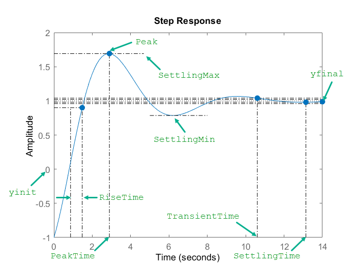
Time constant

At one (\tau):

63%

At 4τ:

almost fully settled

Rise time

T_r=2.2\tau

Time from 10% → 90%

Settling time

T_s=4\tau

Time until stable within ±2%

This is used everywhere in control design.

Page 9 — Impulse Response

For impulse input:

u(s)=1

Response becomes:

y(t)=\frac{K_p}{\tau_p}e^{-t/\tau_p}

This is exponential decay.

Meaning

Impulse gives sudden peak response that decays.

Like hitting a spring.

Very common in system identification.

Page 10 — Ramp Response

For ramp:

u(s)=\frac{1}{s^2}

The output lags behind the ramp.

Important idea:

first-order systems cannot instantly follow changing inputs

They always have delay.

Page 11 — Integrating Systems

This is the second major topic.

\dot{C}(t)=KU(t)

Meaning:

output is integral of input

C(t)=\int U(t)dt

Very intuitive meaning

If input stays positive, output keeps growing forever.

Unlike first-order systems, it does NOT saturate.

Examples

Car

velocity → integrated gives position

x(t)=\int v(t)dt

Tank

flow → integrated gives volume

V(t)=\int f_(t)dt

Very important.

Page 12 — Tank Without Outlet

This is a pure integrator.

Constant inflow gives:

l(t)=\frac{1}{\rho A}t

This means level increases linearly forever.

This is exactly what the graph should look like.

Straight line.

Page 13 — Feedback on Integrator

Very important concept.

When feedback is added:

\frac{K}{s+K}

Suddenly the integrator behaves like a first-order system

This is super important in control design.

Feedback stabilizes integrating systems.

Pages 14–15 — Experimental Parameter Estimation

These slides show how to determine system parameters from real data.

This is system identification.

First-order

From graph:

final value → gain
63% point → τ

Example:

G(s)=\frac{9}{4s+1}

Integrator

Slope gives gain

K=\frac{\Delta y}{\Delta t}

Very practical engineering method.

Page 17–20 — Why Linearization?

This is one of the most important theory parts.

Laplace methods require linear equations.

But real systems are often nonlinear.

So we approximate them locally as linear.

This is called linearization.

Page 21 — Nonlinear Equations

Examples:

5y^2+\sqrt{u}

These are nonlinear because variables multiply or are squared.

Laplace cannot directly solve these.

Pages 23–29 — Linearization (VERY IMPORTANT)

This is Taylor approximation around an operating point.

Core idea:

Approximate nonlinear curve by tangent line locally.

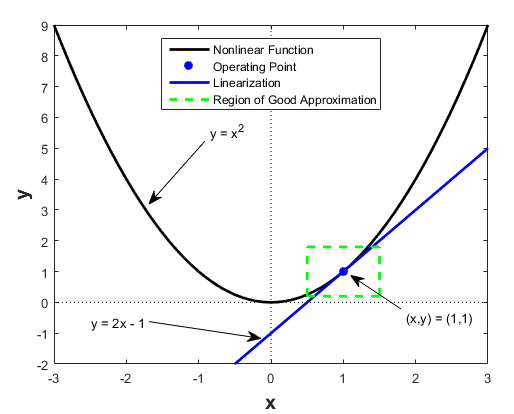
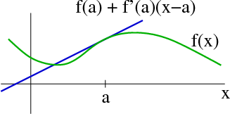
Main idea

Near operating point:

(\bar{y},\bar{u})

small changes:

\hat{y}=y-\bar{y}

\hat{u}=u-\bar{u}

Then system becomes approximately linear.

Why useful?

Because then we can use:

Laplace
transfer functions
control design

This is the foundation of modern control.

Pages 30–34 — Room Temperature Example

This is a full practical example.

Very nice slide.

The room behaves as first-order thermal system.

Model

cm\frac{dT}{dt}=P-hA(T-T_0)

This is exactly same as metal block.

Input:

heater power

Output:

room temperature

Linearization

They define:

\hat{T}=T-20

Meaning:

temperature deviation from 20°C

This makes equation linear.

Very common engineering trick.

Step response

For 1000 W heater:

temperature rises exponentially.

Graph shows room slowly approaching steady state.

Very realistic.

Page 35 — Final Control Structure

Very important concept.

Controller works on small signal deviations, not absolute values.

This is how real controllers are often designed.

Example:

maintain room at 22°C

controller only reacts to deviation from 22°C.

Big Picture Summary

This lecture teaches 3 absolutely core control concepts:

1) First-order systems

\frac{K}{\tau s+1}

Exponential response

63% at τ

2) Integrators

\frac{K}{s}

Output keeps increasing

3) Linearization

Approximate nonlinear systems near operating point

Enables Laplace + control design

This is one of the most foundational lectures in control engineering.

Quiz

Score: 0/30 (0%)

Q0. A first-order system has the transfer function G(s) = K/(τs + 1). What does the time constant τ represent for a step input?

The time required for the output to reach 100% of its final value

The time required for the output to reach approximately 63% of its final value

The time required for the input to become zero

The time required for the system gain to become infinite

Q1. In the metal block heating example, what physical effect is represented by the term hA(Tm(t) - Ts)?

The heat stored inside the metal block

The heat loss from the metal block to the surroundings

The electrical power generated by the metal block

The mass flow rate into the system

Q2. Which transfer function form is characteristic of a pure integrating system?

G(s) = K/(τs + 1)

G(s) = K/s

G(s) = Ks + 1

G(s) = s/K

Q3. For a tank with no outlet and constant inflow, what happens to the liquid level over time?

It approaches a fixed steady-state value exponentially

It oscillates around the initial level

It increases linearly over time

It immediately reaches its maximum value

Q4. What is the Laplace transform of a unit step input?

1/s

1/s^2

Q5. What is the Laplace transform of a unit impulse input?

1/s

1/s^2

s^2

Q6. What is the Laplace transform of a unit ramp input?

1/s

1/s^2

Q7. In the closed-loop transfer function Y(s)/R(s) = D(s)G(s)/(1 + D(s)G(s)H(s)), what does H(s) usually represent?

The process being controlled

The controller

The feedback or measurement element

The external disturbance only

Q8. In experimental identification of a first-order system from a step response, how is the gain K found for a unit step input?

By measuring the slope at time zero only

By measuring the final steady-state output value

By measuring the time where the output reaches 63%

By calculating the area under the impulse input

Q9. If a first-order system has a final value of 9 after a unit step input and reaches 63% of that value at t = 4, what is its transfer function?

G(s) = 4/(9s + 1)

G(s) = 9/(4s + 1)

G(s) = 9/s

G(s) = 4s + 9

Q10. For an integrating system identified experimentally, what does the slope of the output response to a unit step input represent?

The time constant

The system gain K

The pole location only

The feedback sensor gain

Q11. Why is linearization introduced in the lecture?

Because Laplace transformation only works directly for linear differential equations

Because nonlinear systems are always unstable

Because first-order systems cannot be represented using transfer functions

Because integrating systems cannot be controlled

Q12. Which of the following is an example of a nonlinear term?

K1y(t) + K2u(t)

5y(t)

y(t)u(t)

3u(t)

Q13. In linearization, what does a hatted variable such as ŷ(t) usually represent?

The absolute value of the output

The output at infinite time

The deviation from the operating point

The nonlinear part of the input only

Q14. When feedback control is applied to a pure integrating system with plant 1/s and controller gain K, what type of closed-loop system results?

A second-order oscillating system

A first-order system

A pure differentiator

An unstable open-loop system

Q15. A first-order system reaches approximately 63% of its final value after one time constant.

True

False

Q16. A pure integrating system always approaches a fixed final value after a constant step input.

True

False

Q17. The transfer function G(s) = K/(τs + 1) is a standard form for a first-order system.

True

False

Q18. The Laplace transform method can be directly applied to any nonlinear differential equation without approximation.

True

False

Q19. In the room temperature example, heater power P(t) is treated as an input and room temperature T(t) as the output.

True

False

Q20. In the tank example without outlet, the liquid level behaves like a first-order system with an exponential step response.

True

False

Q21. Linearization approximates a nonlinear system near an operating point.

True

False

Q22. The operating point values are usually written with bars, such as ȳ and ū.

True

False

Q23. For a first-order system, a larger time constant τ generally means a faster response.

True

False

Q24. In the closed-loop transfer function, the denominator 1 + D(s)G(s)H(s) contains the effect of feedback.

True

False

Q25. A ramp input has Laplace transform 1/s^2.

True

False

Q26. For a first-order step response, the output starts at the final value and then decays to zero.

True

False

Q27. In the room temperature linearization example, T̂(t) represents the deviation of the room temperature from the operating point temperature.

True

False

Q28. If the input step used for experimental identification is not equal to 1, the gain K is found by dividing the final output change by the input step size.

True

False

Q29. A nonlinear function can be approximated locally by using the slope at the operating point.

True

False