Laplace Transformation and Modelling — Full Slide Summary

This lecture is really about how we model real physical systems mathematically and then make them easier to solve using Laplace transforms.

A big idea throughout the slides is this:

Real systems are described by differential equations Laplace transforms convert them into algebra equations Algebra is much easier to solve

This is one of the most important ideas in control engineering.

Page 1 — Title

Laplace transformation and a bit more modelling

This lecture combines two major topics:

• Laplace transforms
• mathematical modelling of physical systems

These two always go together in control theory.

Page 2 — Detailed functional block diagram

This page shows a real-world control loop implementation.

The flow is:

• reference / desired value
• controller algorithm
• D/A or PWM conversion
• actuator
• physical system
• sensor
• A/D conversion
• feedback back to controller

This is basically how a real embedded system works.

Example:

• desired temperature = 37°C
• controller compares actual vs desired
• sends voltage to heater
• sensor measures actual temperature
• repeats continuously

This is the practical engineering version of control systems.

Page 3 — Standard feedback setup

This is the classic feedback loop.

The main components:

• reference = what you want
• controller = decides correction
• plant/system = physical thing being controlled
• sensor = measures output
• feedback loop = compares output to reference

The error is:

\text{Error} = \text{Reference} - \text{Measured output}

This error drives the controller.

This page is extremely important.

This structure appears everywhere:

• cruise control
• thermostat
• robot arm
• tank level control
• fermentor temperature

Page 4 — Solving linear differential equations

This slide introduces the core workflow.

Time domain:

\frac{dy}{dt}=f(y)

This is hard to solve directly for complex systems.

Laplace transform converts it into:

sY(s)-y(0)=F(s)

Now it becomes algebra.

That is MUCH easier.

So workflow becomes:

Differential equation → Laplace → algebra → inverse Laplace → time response

This is the entire purpose of Laplace.

Page 5 — Why Laplace is useful

This slide explains why we need it.

Real systems often have:

• multiple subsystems
• coupled equations
• different orders
• time-dependent inputs

These are very hard to solve directly.

Laplace lets us solve each subsystem separately.

Then combine them using algebra.

This is the foundation of block-diagram control.

Page 6 — Same workflow repeated

This slide reinforces the transformation flow.

Very important concept:

Laplace changes dynamic systems into static equations.

That means instead of derivatives, we work with multiplication by (s).

That is the magic.

Page 7 — Laplace definition

Here is the formal definition:

F(s)=\int_0^{\infty} f(t)e^{-st},dt

Where:

s=\sigma + j\omega

This means (s) is a complex frequency variable.

Do not worry too much yet about the complex part.

For most control problems, think of (s) as a mathematical variable that replaces differentiation.

The exponential term:

e^{-st}

acts as a weighting function.

Page 8 — Typical examples

This page is SUPER important.

Common Laplace pairs:

1 \leftrightarrow \frac{1}{s}

constant function

t^n \leftrightarrow \frac{n!}{s^{n+1}}

polynomials

\sin(at)\leftrightarrow \frac{a}{s^2+a^2}

oscillations

These are formulas you often memorize.

Pages 9–10 — Laplace tables

These pages are basically formula sheets.

Very important entries:

First derivative:

\mathcal{L}\left{\frac{dy}{dt}\right}=sY(s)-y(0)

Second derivative:

\mathcal{L}\left{\frac{d^2y}{dt^2}\right}=s^2Y(s)-sy(0)-y'(0)

Exponential:

e^{-\alpha t}\leftrightarrow \frac{1}{s+\alpha}

Step input:

1(t)\leftrightarrow \frac{1}{s}

These are used constantly in controller design.

Page 11 — Common rules

Important modelling rules.

Superposition

\mathcal{L}(af_1+bf_2)=aF_1+bF_2

This means Laplace is linear.

Very important because linear systems can be split into parts.

Time delay

f(t-\gamma)\leftrightarrow e^{-s\gamma}F(s)

This is extremely useful.

A delay in time becomes exponential multiplication.

Used in:

• transport delay
• sensor delay
• communication delay

Page 12 — Differentiation and integration

Key formulas:

Differentiation:

\mathcal{L}\left{\frac{df}{dt}\right}=sF(s)-f(0)

Integration:

\mathcal{L}\left{\int_0^t f(\theta)d\theta\right}=\frac{1}{s}F(s)

This second one is very important:

integration in time = division by (s)

Page 13 — Transfer functions

This is one of the most important concepts.

A transfer function is:

G(s)=\frac{Y(s)}{U(s)}

output over input

assuming zero initial conditions.

This tells you how the system behaves.

It is basically the mathematical identity of a system.

Page 14 — Standard setup in Laplace domain

Same feedback loop but now everything is in transfer function form.

Blocks:

• controller = (D(s))
• plant = (G(s))
• sensor = (H(s))

This lets you use algebra instead of differential equations.

Extremely powerful.

Page 15 — Example I

Given:

\frac{dM}{dt}=F(t)-KM(t)

This is a first-order system.

Laplace gives:

sM(s)=F(s)-KM(s)

Rearrange:

\frac{M(s)}{F(s)}=\frac{1}{s+K}

This is the transfer function.

For (K=2):

\frac{1}{s+2}

Classic first-order system.

Pages 16–18 — Inverse Laplace and step response

Inverse Laplace converts back to time.

For:

\frac{1}{s+2}

time response is:

e^{-2t}

For step input:

F(s)=\frac{1}{s}

response becomes:

\frac{1}{s(s+2)}

inverse gives:

1-e^{-2t}

This is the standard first-order rise curve.

Very important shape.

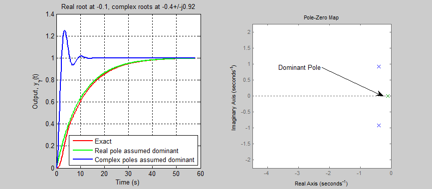
This curve approaches steady state gradually.

Pages 19–22 — Block diagram algebra

This is extremely important.

The “golden formula”:

\frac{Y(s)}{R(s)}=\frac{D(s)G(s)}{1+D(s)G(s)H(s)}

This is the closed-loop transfer function.

Memorize this.

Meaning:

• numerator = direct path
• denominator = feedback correction

This is the heart of feedback control.

Page 23 — Break

Just a lecture pause slide.

Page 24 — Mass balance

Now we move into modelling.

Very important physical law:

mass cannot be created or destroyed

So:

\frac{dM}{dt}=F_-F_

This is conservation of mass.

This equation is used in:

• tanks
• reactors
• fermentors
• fluid systems

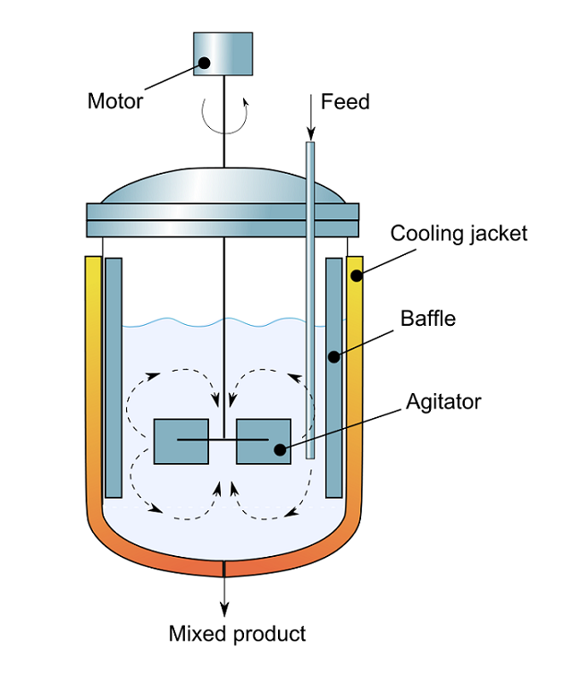
Page 25 — Two-component mixing

This image-only slide is very important.

It shows two components mixing in a control volume.

Concentration:

c=\frac{M_1}{M_1+M_2}

This means fraction of component 1.

The differential equations describe how each component changes over time.

This is classic mixing-tank modelling.

Page 26 — Mass balance with reaction

Now reaction is added.

So balance becomes:

\text{in} - \text{out} \pm \text{reaction}

This is a reactor model.

Component 1 decreases:

-F_

Component 2 increases:

+F_

This is conservation with conversion.

Pages 27–29 — Reaction example

Reaction rate:

F_=KM_1

This is first-order kinetics.

Very common in:

• chemical engineering
• pharmacokinetics
• biology

The resulting transfer function:

\frac{M(s)}{F(s)}=\frac{1}{s+K}

Again first-order dynamics.

This shows how physical systems often reduce to the same mathematical structure.

Very important insight.

Page 30 — Level model

This is a liquid tank model.

\frac{dh}{dt}=K_t(q_i-q_o)

Height changes depending on flow difference.

This is extremely intuitive.

If inflow > outflow:

level rises

If inflow < outflow:

level drops

Laplace gives:

h(s)=\frac{K_t}{s}(q_i-q_o)

Notice division by (s).

This means:

tank level is an integrator

This is a major control concept.

Page 31 — First law of thermodynamics

Energy balance:

\Delta U = Q + W

Change in internal energy equals:

• heat added
• work done

This is conservation of energy.

The image explains heat and work flowing into the system.

Very useful for temperature modelling.

Pages 32–33 — Fermentor temperature model

Very important practical example.

Two coupled first-order systems:

• heater shell
• fermentor liquid

Each has its own time constant.

This creates a second-order response.

Transfer function becomes product of two first-order blocks:

\frac{K_U}{\tau_Us+1}\cdot \frac{K_F}{\tau_Fs+1}

This means the system responds slower than a single block.

The difference of exponentials in time domain is classic second-order behavior.

Page 34 — MATLAB simulation

This slide shows simulation.

Very useful.

A = 3/(s+3)
B = 0.5/(s+0.5)
C = A*B

This means:

• A = heater → shell
• B = shell → liquid
• C = total system

Then step(C) plots the step response.

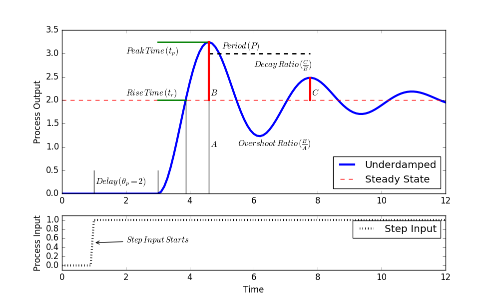
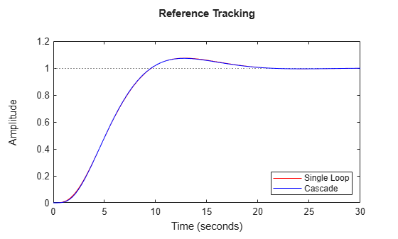
The graph shows:

• fastest response = A
• slower = B
• slowest = combined C

Exactly what we expect physically.

Big-picture takeaway

This whole lecture teaches one master idea:

Build physical models with conservation laws Convert them into differential equations Use Laplace transforms to solve and analyze them

This is the mathematical foundation of control engineering.